NLP for Task Classification
25 Sep 2017
. category:
Portfolio Building
.
Comments
UPDATE 11/17/2017: I wrote a follow-up post about deploying this model to a web service via Azure ML - check it out!
Everything between this sentence and the Wrap Up section has been converted from my nlp_classifier notebook1 on GitHub.
Notebook
Hypothesis: Part of Speech (POS) tagging and syntactic dependency parsing provides valuable information for classifying imperative phrases. The thinking is that being able to detect imperative phrases will transfer well to detecting tasks and to-dos.
Some Terminology
- Imperative mood is "used principally for ordering, requesting or advising the listener to do (or not to do) something... also often used for giving instructions as to how to perform a task."
- Part of speech (POS) is a way of categorizing a word based on its syntactic function.
- The POS tagger from Spacy.io that is used in this notebook differentiates between pos_ and tag_ - POS (pos_) refers to "coarse-grained part-of-speech" like
VERB,ADJ, orPUNCT; and POSTAG (tag_) refers to "fine-grained part-of-speech" likeVB,JJ, or..
- The POS tagger from Spacy.io that is used in this notebook differentiates between pos_ and tag_ - POS (pos_) refers to "coarse-grained part-of-speech" like
- Syntactic dependency parsing is a way of connecting words based on syntactic relationships, such as
DOBJ(direct object),PREP(prepositional modifier), orPOBJ(object of preposition).- Check out the dependency parse of the phrase "Send the report to Kyle by tomorrow" as an example.
Proposed Features
The imperative mood centers around actions, and actions are generally represented in English using verbs. So the features are engineered to also center on the VERB:
FeatureName.VERB: Does the phrase containVERB(s) of the tag formVB*?FeatureName.FOLLOWING_POS: Are the words following theVERB(s) of certain parts of speech?FeatureName.FOLLOWING_POSTAG: Are the words following theVERB(s) of certain POS tags?FeatureName.CHILD_DEP: Are theVERB(s) parents of certain syntactic dependencies?FeatureName.PARENT_DEP: Are theVERB(s) children of certain syntactic dependencies?FeatureName.CHILD_POS: Are the syntactic dependencies that theVERB(s) are children of of certain parts of speech?FeatureName.CHILD_POSTAG: Are the syntactic dependencies that theVERB(s) are children of of certain POS tags?FeatureName.PARENT_POS: Are the syntactic dependencies that theVERB(s) parent of certain parts of speech?FeatureName.PARENT_POSTAG: Are the syntactic dependencies that theVERB(s) parent of certain POS tags?
Notes:
- Features 2-9 all depend on feature 1 between
True; ifFalse, phrase vectorization will result in all zeroes. - When features 2-9 are applied to actual phrases, they will append identifying informating about the feature in the form of
_*(e.g.,FeatureName.FOLLOWING_POSTAG_WRB).
Data and Setup
Building a recipe corpus
I wrote and ran epicurious_recipes.py* to scrape Epicurious.com for recipe instructions and descriptions. I then performed some manual cleanup of the script results. Output is in epicurious-pos.txt and epicurious-neg.txt.
* script (very) loosely based off of https://github.com/benosment/hrecipe-parse
Note that deriving all negative examples in the training set from Epicurious recipe descriptions would result in negative examples that are longer and syntactically more complicated than the positive examples. This is a form of bias.
To (hopefully?) correct for this a bit, I will add the short movie reviews found at https://pythonprogramming.net/static/downloads/short_reviews/ as more negative examples.
This still feels weird because we're selecting negative examples only from specific categories of text (recipe descriptions, short movie reviews) - just because they're readily available. Further, most positive examples are recipe instructions - also a specific (and not necessarily related to the main "task" category) category of text.
Ultimately though, this recipe corpus is a stopgap/proof of concept for a corpus more relevant to tasks later on, so I won't worry further about this for now.
import os
from pandas import read_csv
from numpy import random
BASE_DIR = os.getcwd()
data_path = BASE_DIR + '/data.tsv'
df = read_csv(data_path, sep='\t', header=None, names=['Text', 'Label'])
df.head()
pos_data_split = list(df.loc[df.Label == 'pos'].Text)
neg_data_split = list(df.loc[df.Label == 'neg'].Text)

num_pos = len(pos_data_split)
num_neg = len(neg_data_split)

# 50/50 split between the number of positive and negative samples
num_per_class = num_pos if num_pos < num_neg else num_neg

# shuffle samples
random.shuffle(pos_data_split)
random.shuffle(neg_data_split)
lines = []
for l in pos_data_split[:num_per_class]:
    lines.append((l, 'pos'))
for l in neg_data_split[:num_per_class]:
    lines.append((l, 'neg'))
# Features as defined in the introduction
from enum import Enum, auto
class FeatureName(Enum):
    VERB = auto()
    FOLLOWING_POS = auto()
    FOLLOWING_POSTAG = auto()
    CHILD_DEP = auto()
    PARENT_DEP = auto()
    CHILD_POS = auto()
    CHILD_POSTAG = auto()
    PARENT_POS = auto()
    PARENT_POSTAG = auto()
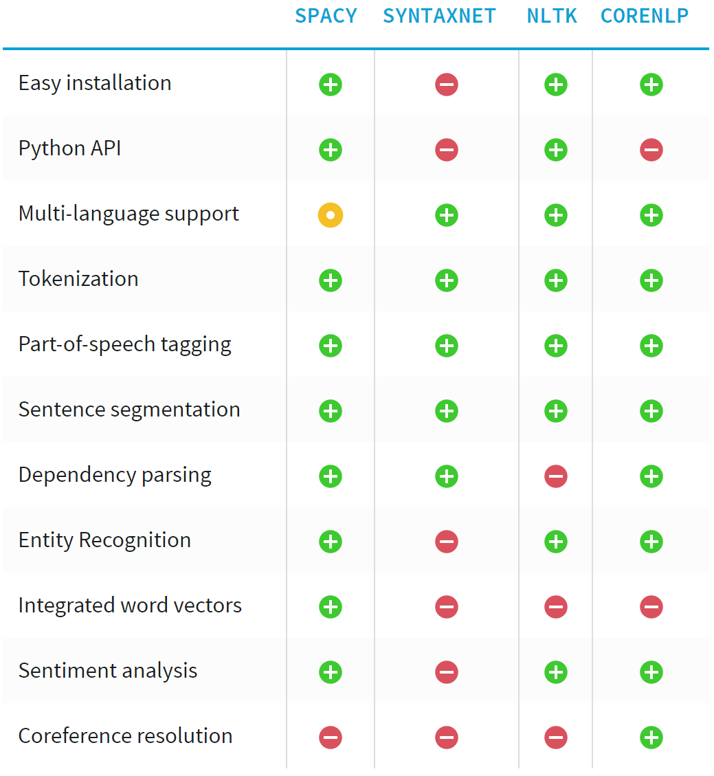
spaCy.io for NLP
Because Stanford CoreNLP is hard to install for Python
Found Spacy through an article on "Training a Classifier for Relation Extraction from Medical Literature" (GitHub)
#!conda config --add channels conda-forge
#!conda install spacy
#!python -m spacy download en
Using the Spacy Data Model for NLP
import spacy
# slow
nlp = spacy.load('en')
Spacy's sentence segmentation is lacking... https://github.com/explosion/spaCy/issues/235. So each '\n' will start a new Spacy Doc.
def create_spacy_docs(ll):
    dd = [(nlp(l[0]), l[1]) for l in ll]
    # collapse noun phrases into single compounds
    for d in dd:
        for np in d[0].noun_chunks:
            np.merge(np.root.tag_, np.text, np.root.ent_type_)
    return dd
# slower
docs = create_spacy_docs(lines)
NLP output
Tokenization, POS tagging, and dependency parsing happened automatically with the nlp(line) calls above! So let's look at the outputs.
https://spacy.io/docs/usage/data-model and https://spacy.io/docs/api/doc will be useful going forward
for doc in docs[:10]:
    print(list(doc[0].sents))
for doc in docs[:10]:
    print(list(doc[0].noun_chunks))
for doc in docs[:5]:
    for token in doc[0]:
        print(token.text, token.dep_, token.lemma_, token.pos_, token.tag_, token.head, list(token.children))
Featurization
import re
from collections import defaultdict

def featurize(d):
    s_features = defaultdict(int)
    for idx, token in enumerate(d):
        if re.match(r'VB.?', token.tag_) is not None: # note: not using token.pos == VERB because this also includes BES, HVS, MD tags
            s_features[FeatureName.VERB.name] += 1
            # FOLLOWING_POS
            # FOLLOWING_POSTAG
            next_idx = idx + 1;
            if next_idx < len(d):
                s_features[f'{FeatureName.FOLLOWING_POS.name}_{d[next_idx].pos_}'] += 1
                s_features[f'{FeatureName.FOLLOWING_POSTAG.name}_{d[next_idx].tag_}'] += 1
            # PARENT_DEP
            # PARENT_POS
            # PARENT_POSTAG
            '''
            "Because the syntactic relations form a tree, every word has exactly one head.
            You can therefore iterate over the arcs in the tree by iterating over the words in the sentence."
            https://spacy.io/docs/usage/dependency-parse#navigating
            '''
            if (token.head is not token):
                s_features[f'{FeatureName.PARENT_DEP.name}_{token.head.dep_.upper()}'] += 1
                s_features[f'{FeatureName.PARENT_POS.name}_{token.head.pos_}'] += 1
                s_features[f'{FeatureName.PARENT_POSTAG.name}_{token.head.tag_}'] += 1
            # CHILD_DEP
            # CHILD_POS
            # CHILD_POSTAG
            for child in token.children:
                s_features[f'{FeatureName.CHILD_DEP.name}_{child.dep_.upper()}'] += 1
                s_features[f'{FeatureName.CHILD_POS.name}_{child.pos_}'] += 1
                s_features[f'{FeatureName.CHILD_POSTAG.name}_{child.tag_}'] += 1
    return dict(s_features)
featuresets = [(doc[0], (featurize(doc[0]), doc[1])) for doc in docs]
from statistics import mean, median, mode, stdev
f_lengths = [len(fs[1][0]) for fs in featuresets]

print('Stats on number of features per example:')
print(f'mean: {mean(f_lengths)}')
print(f'stdev: {stdev(f_lengths)}')
print(f'median: {median(f_lengths)}')
print(f'mode: {mode(f_lengths)}')
print(f'max: {max(f_lengths)}')
print(f'min: {min(f_lengths)}')
featuresets[:2]
On one run, the above line printed the following featureset:
(Gather foil loosely on top and bake for 1 1/2 hours., ({}, 'pos'))
This is because the Spacy.io POS tagger provided this:
Gather/NNP foil/NN loosely/RB on/IN top/NN and/CC bake/NN for/IN 1 1/2 hours./NNS
...with no VERBs tagged, which is incorrect.
"Voting - POS taggers and classifiers" in the Next Steps/Improvements section below is meant to improve on this.
Compare to Stanford CoreNLP POS tagger:
Gather/VB foil/NN loosely/RB on/IN top/JJ and/CC bake/VB for/IN 1 1/2/CD hours/NNS ./.
And Stanford Parser:
Gather/NNP foil/VB loosely/RB on/IN top/NN and/CC bake/VB for/IN 1 1/2/CD hours/NNS ./.
Classification
random.shuffle(featuresets)

num_classes = 2
split_num = round(num_per_class*num_classes / 5)

# train and test sets
testing_set = [fs[1] for i, fs in enumerate(featuresets[:split_num])]
training_set =  [fs[1] for i, fs in enumerate(featuresets[split_num:])]

print(f'# training samples: {len(training_set)}')
print(f'# test samples: {len(testing_set)}')
# decoupling the functionality of nltk.classify.accuracy
def predict(classifier, gold, prob=True):
    if (prob is True):
        predictions = classifier.prob_classify_many([fs for (fs, ll) in gold])
    else:
        predictions = classifier.classify_many([fs for (fs, ll) in gold])
    return list(zip(predictions, [ll for (fs, ll) in gold]))

def accuracy(predicts, prob=True):
    if (prob is True):
        correct = [label == prediction.max() for (prediction, label) in predicts]
    else:
        correct = [label == prediction for (prediction, label) in predicts]

    if correct:
        return sum(correct) / len(correct)
    else:
        return 0
Note below the use of DummyClassifier to provide a simple sanity check, a baseline of random predictions. stratified means it "generates random predictions by respecting the training set class distribution." (http://scikit-learn.org/stable/modules/model_evaluation.html#dummy-estimators)
More generally, when the accuracy of a classifier is too close to random, it probably means that something went wrong: features are not helpful, a hyperparameter is not correctly tuned, the classifier is suffering from class imbalance, etc…
If a classifier can beat the DummyClassifier, it is at least learning something valuable! How valuable is another question...
from nltk import NaiveBayesClassifier
from nltk.classify.decisiontree import DecisionTreeClassifier
from nltk.classify.scikitlearn import SklearnClassifier

from sklearn.dummy import DummyClassifier
from sklearn.naive_bayes import MultinomialNB, BernoulliNB
from sklearn.linear_model import LogisticRegressionCV, SGDClassifier
from sklearn.svm import SVC, LinearSVC
from sklearn.ensemble import RandomForestClassifier
from sklearn.calibration import CalibratedClassifierCV

dummy = SklearnClassifier(DummyClassifier(strategy='stratified', random_state=0))
dummy.train(training_set)
dummy_predict = predict(dummy, testing_set)
dummy_accuracy = accuracy(dummy_predict)
print("Dummy classifier accuracy percent:", dummy_accuracy*100)

nb = NaiveBayesClassifier.train(training_set)
nb_predict = predict(nb, testing_set)
nb_accuracy = accuracy(nb_predict)
print("NaiveBayes classifier accuracy percent:", nb_accuracy*100)

multinomial_nb = SklearnClassifier(MultinomialNB())
multinomial_nb.train(training_set)
mnb_predict = predict(multinomial_nb, testing_set)
mnb_accuracy = accuracy(mnb_predict)
print("MultinomialNB classifier accuracy percent:", mnb_accuracy*100)

bernoulli_nb = SklearnClassifier(BernoulliNB())
bernoulli_nb.train(training_set)
bnb_predict = predict(bernoulli_nb, testing_set)
bnb_accuracy = accuracy(bnb_predict)
print("BernoulliNB classifier accuracy percent:", bnb_accuracy*100)

# ??logistic_regression._clf
#   sklearn.svm.LinearSVC : learns SVM models using the same algorithm.
logistic_regression = SklearnClassifier(LogisticRegressionCV())
logistic_regression.train(training_set)
lr_predict = predict(logistic_regression, testing_set)
lr_accuracy = accuracy(lr_predict)
print("LogisticRegressionCV classifier accuracy percent:", lr_accuracy*100)

# ??sgd._clf
#    The 'log' loss gives logistic regression, a probabilistic classifier.
# ??linear_svc._clf
#   can optimize the same cost function as LinearSVC
#   by adjusting the penalty and loss parameters. In addition it requires
#   less memory, allows incremental (online) learning, and implements
#   various loss functions and regularization regimes.
sgd = SklearnClassifier(SGDClassifier(loss='log'))
sgd.train(training_set)
sgd_predict = predict(sgd, testing_set)
sgd_accuracy = accuracy(sgd_predict)
print("SGD classifier accuracy percent:", sgd_accuracy*100)

# slow
# using libsvm with kernel 'rbf' (radial basis function)
svc = SklearnClassifier(SVC(probability=True))
svc.train(training_set)
svc_predict = predict(svc, testing_set)
svc_accuracy = accuracy(svc_predict)
print("SVC classifier accuracy percent:", svc_accuracy*100)

# ??linear_svc._clf
#    Similar to SVC with parameter kernel='linear', but implemented in terms of
#    liblinear rather than libsvm, so it has more flexibility in the choice of
#    penalties and loss functions and should scale better to large numbers of
#    samples.
#    Prefer dual=False when n_samples > n_features.
# Using CalibratedClassifierCV as wrapper to get predict probabilities (https://stackoverflow.com/a/39712590)
linear_svc = SklearnClassifier(CalibratedClassifierCV(LinearSVC(dual=False)))
linear_svc.train(training_set)
linear_svc_predict = predict(linear_svc, testing_set)
linear_svc_accuracy = accuracy(linear_svc_predict)
print("LinearSVC classifier accuracy percent:", linear_svc_accuracy*100)

# slower
dt = DecisionTreeClassifier.train(training_set)
dt_predict = predict(dt, testing_set, False)
dt_accuracy = accuracy(dt_predict, False)
print("DecisionTree classifier accuracy percent:", dt_accuracy*100)

random_forest = SklearnClassifier(RandomForestClassifier(n_estimators = 100))
random_forest.train(training_set)
rf_predict = predict(random_forest, testing_set)
rf_accuracy = accuracy(rf_predict)
print("RandomForest classifier accuracy percent:", rf_accuracy*100)
SGD: Multiple Epochs
sgd classifiers improves with epochs. ??sgd._clf tells us that the default number of epochs n_iter is 5. So let's run more epochs. Also not that the training_set shuffle is True by default.
num_epochs = 1000
sgd = SklearnClassifier(SGDClassifier(loss='log', n_iter=num_epochs))
sgd.train(training_set)
sgd_predict = predict(sgd, testing_set)
sgd_accuracy = accuracy(sgd_predict)
print(f"SGDClassifier classifier accuracy percent (epochs: {num_epochs}):", sgd_accuracy*100)
Fortunately, 1000 epochs run very quickly! And SGDClassifier performance has improved with more iterations.
Also note that we can set warm_start to True if we want to take advantage of online learning and reuse the solution of the previous call.
GridSearch and Cross-Validation
Next we perform 1) grid search to find optimal hyperparameters, and 2) cross-validation to evaluate performance over multiple folds of the data (to avoid overfitting).
http://scikit-learn.org/stable/modules/grid_search.html#grid-search
http://scikit-learn.org/stable/auto_examples/model_selection/plot_nested_cross_validation_iris.html
from nltk.classify.scikitlearn import SklearnClassifier

from sklearn.linear_model import SGDClassifier
from sklearn.svm import LinearSVC
from sklearn.ensemble import RandomForestClassifier
from sklearn.calibration import CalibratedClassifierCV
# https://stackoverflow.com/a/16388804
from sklearn.model_selection import KFold
from sklearn.base import clone
from numpy import zeros

def cross_val(name, model, debug=True):
    num_splits = 3
    original_clf = clone(model._clf)
    cvidx = KFold(n_splits=num_splits, shuffle=True).split(training_set)

    nested_acc = zeros(num_splits)
    i=0
    for trainidx, testidx in cvidx:
        model._clf = clone(original_clf)  # we clone the estimator to make sure that all the folds are independent
        classifier = model.train(training_set[trainidx[0]:trainidx[len(trainidx)-1]])
        pred = predict(classifier, training_set[testidx[0]:testidx[len(testidx)-1]])
        nested_acc[i] = accuracy(pred)
        i += 1

    if debug == True:
        print(f"{name} CV accuracies:", nested_acc)

    return nested_acc.mean()
# http://scikit-learn.org/stable/auto_examples/model_selection/plot_grid_search_digits.html#sphx-glr-auto-examples-model-selection-plot-grid-search-digits-py

from sklearn.model_selection import GridSearchCV
from sklearn.linear_model import LogisticRegression

# Set the parameters by cross-validation
model_parameters = [{'LinearSVC': [{
                        'loss': ['hinge'],
                        'dual': [True],
                        'penalty': ['l2'],
                        'tol': [1e-3, 1e-4, 1e-5],
                        'max_iter': [1000, 10000],
                        'C': [100.0, 1.0, 0.01]
                    },
                    {
                        'loss': ['squared_hinge'],
                        'dual': [False, True],
                        'penalty': ['l2'],
                        'tol': [1e-3, 1e-4, 1e-5],
                        'max_iter': [1000, 10000],
                        'C': [100.0, 1.0, 0.01]
                    }]},
                   {'LogisticRegression': [{
                        'penalty': ['l1'],
                        'dual': [False],
                        'C': [100.0, 1.0, 0.01],
                        'solver': ['liblinear']
                   },
                   {
                        'penalty': ['l2'],
                        'dual': [False, True],
                        'C': [100.0, 1.0, 0.01],
                        'max_iter': [100, 1000],
                        'solver': ['liblinear'],
                        'tol': [1e-3, 1e-4, 1e-5]
                   },
                   {
                        'penalty': ['l2'],
                        'dual': [False],
                        'C': [100.0, 1.0, 0.01],
                        'max_iter': [100, 1000],
                        'solver': ['newton-cg', 'lbfgs', 'sag'],
                        'tol': [1e-3, 1e-4, 1e-5]
                   }]},
                   {'SGD': [{
                        'penalty': ['l1', 'l2', 'elasticnet'],
                        'alpha': [1e-3, 1e-4, 1e-5],
                        'average': [True, False],
                        'n_iter': [100, 1000, 10000]
                   }]},
                   {'RandomForest': [{
                        'n_estimators': [10, 100, 1000],
                        'criterion': ['gini', 'entropy'],
                        'max_features': ['auto', 'log2', None],
                        'oob_score': [True, False]
                   }]}]

score = 'roc_auc'

for i, model_param in enumerate(model_parameters):
    model = [key for i, key in enumerate(model_param)][0]

    print(f"# {model}: Tuning hyper-parameters for {score}")
    print()

    if model == 'LinearSVC':
        clf = LinearSVC()
    elif model == 'LogisticRegression':
        clf = LogisticRegression()
    elif model == 'SGD':
        clf = SGDClassifier(loss='log')
    elif model == 'RandomForest':
        clf = RandomForestClassifier()
    else:
        raise Exception('%s model needs to be added to the if-block' % model)

    grid = SklearnClassifier(GridSearchCV(clf, model_param[model], cv=5,
                       scoring=score, n_jobs=-1))
    grid.train(training_set)

    print("Best parameters set found on development set:")
    print()
    print(grid._clf.best_params_)
    mean = grid._clf.cv_results_['mean_test_score'][grid._clf.best_index_]
    std = grid._clf.cv_results_['std_test_score'][grid._clf.best_index_]
    print("roc_auc: %0.3f (+/-%0.03f)" % (mean, std * 2))
    print()

    if model == 'LinearSVC':
        # Wrapping LinearSVC in CalibratedClassifierCV to add support for probability prediction
        # Note that there is a difference in accuracies between raw GridSearchCV and calibrated GridSearchCV
        # However, I'm willing to sacrifice the potential 'best' result from raw in order to output probabilities
        grid_calibrated = SklearnClassifier(CalibratedClassifierCV(grid._clf.best_estimator_, cv=None))
        grid_calibrated.train(training_set)
        gridc_predict = predict(grid_calibrated, testing_set)
        gridc_accuracy = accuracy(gridc_predict)
        print(f"{model} (calibrated) classifier accuracy percent:", gridc_accuracy*100)

        grid_predict = predict(grid, testing_set, False)
        grid_accuracy = accuracy(grid_predict, False)
        print(f"{model} (raw) classifier accuracy percent:", grid_accuracy*100)

        # CV after parameter optimization
        cv_acc = cross_val(model, grid_calibrated)
        print(f"{model} (calibrated) CV classifier avg accuracy percent:", cv_acc*100)

        linear_svc_opt = grid_calibrated
        linear_svc_predict = gridc_predict
    else:
        grid_predict = predict(grid, testing_set)
        grid_accuracy = accuracy(grid_predict)
        print(f"{model} classifier accuracy percent:", grid_accuracy*100)

        # CV after parameter optimization
        cv_acc = cross_val(model, grid)
        print(f"{model} CV classifier avg accuracy percent:", cv_acc*100)

        if model == 'LogisticRegression':
            logistic_regression_opt = grid
            lr_predict = grid_predict
        elif model == 'SGD':
            sgd_opt = grid
            sgd_predict = grid_predict
        elif model == 'RandomForest':
            random_forest_opt = grid
            rf_predict = grid_predict
        else:
            raise Exception('%s model was not run through Grid Search' % model)

    print()
VotingClassifier
We're going to create an ensemble classifier by letting our top-performing classifiers, which consistently perform with >80% accuracy — LogisticRegression, LinearSVC, SGD, and RandomForest (excluding SVC due to its slowness) — vote on each prediction.
from sklearn.ensemble import VotingClassifier

voting = SklearnClassifier(VotingClassifier(estimators=[
    ('lr', logistic_regression_opt._clf),
    ('linear_svc', linear_svc_opt._clf),
    ('sgd', sgd_opt._clf),
    ('rf', random_forest_opt._clf)
], voting='soft', weights=[1,1,1,3], n_jobs=-1))
voting.train(training_set)

voting_predict = predict(voting, testing_set)
voting_accuracy = accuracy(voting_predict)
print("Soft voting classifier accuracy percent:", voting_accuracy*100)

# CV after parameter optimization
voting_acc = cross_val("Soft voting", voting)
print(f"Soft voting CV classifier accuracy percent:", voting_acc*100)
Analysis
Similarly to the voting model, we're also going to scope analysis down to our top-performing classifiers. We'll include the Voting model itself, and then Dummy as a baseline.
Most Informative Features
# https://stackoverflow.com/a/11140887
def show_most_informative_features(vectorizer, clf, n=20):
    feature_names = vectorizer.get_feature_names()
    coefs_with_fns = sorted(zip(clf.coef_[0], feature_names))
    top = zip(coefs_with_fns[:round(n/2)], coefs_with_fns[:-(round(n/2) + 1):-1])
    for (coef_1, fn_1), (coef_2, fn_2) in top:
        print("\t%.4f\t%-15s\t\t%.4f\t%-15s" % (coef_1, fn_1, coef_2, fn_2))
print('SGD')
show_most_informative_features(sgd._vectorizer, sgd._clf, 15)
print()
print('Logistic Regression')
show_most_informative_features(logistic_regression._vectorizer, logistic_regression._clf, 15)
Note: Because CalibratedClassifierCV has no attribute coef_, we cannot show the most informative features for LinearSVC while it's wrapped. Random Forest and Voting also lack coef_.
spacy.explain("JJS")
Negative coefficients:
- VERB parents
AGENT: "used for agents of passive verbs" - interpreting this to mean that existence of passive verbs (i.e., the opposite of active verbs) means negative correlation with it being imperative - VERB followed by a
WRB: "wh-adverb" (where, when) - VERB is a child of
AMOD: "any adjective or adjectival phrase that serves to modify the meaning" of the verb
Positive coefficients:
- VERB parents a
-RRB-: "right round bracket" - VERB is a child of
PROPN: "proper noun" - VERB is a child of
NNP: "noun, proper singular"
Scikit Learn metrics: Confusion matrix, Classification report, F1 score, Log loss
http://scikit-learn.org/stable/modules/model_evaluation.html
from sklearn import metrics

def classification_report(predict, prob=True):
    predictions, labels = zip(*predict)
    if prob is True:
        return metrics.classification_report(labels, [p.max() for p in predictions])
    else:
        return metrics.classification_report(labels, predictions)

def confusion_matrix(predict, prob=True, print_layout=False):
    predictions, labels = zip(*predict)
    if print_layout is True:
        print('Layout\n[[tn   fp]\n [fn   tp]]\n')
    if prob is True:
        return metrics.confusion_matrix(labels, [p.max() for p in predictions])
    else:
        return metrics.confusion_matrix(labels, predictions)

def log_loss(predict):
    predictions, labels = zip(*predict)
    return metrics.log_loss(labels, [p.prob('pos') for p in predictions])

def roc_auc_score(predict):
    predictions, labels = zip(*predict)
    # need to convert labels to binary classification of 0 or 1
    return metrics.roc_auc_score([1 if l == 'pos' else 0 for l in labels], [p.prob('pos') for p in predictions], average='weighted')

def precision_recall_curve(predict):
    predictions, labels = zip(*predict)
    return metrics.precision_recall_curve(labels, [p.prob('pos') for p in predictions], pos_label='pos')

def average_precision_score(predict):
    predictions, labels = zip(*predict)
    return metrics.average_precision_score([1 if l == 'pos' else 0 for l in labels], [p.prob('pos') for p in predictions])

def roc_curve(predict):
    predictions, labels = zip(*predict)
    return metrics.roc_curve(labels, [p.prob('pos') for p in predictions], pos_label='pos')
print('SGD')
print(classification_report(sgd_predict))
print()
print('Logistic Regression')
print(classification_report(lr_predict))
print()
print('LinearSVC')
print(classification_report(linear_svc_predict))
print()
print('Random Forest')
print(classification_report(rf_predict))
print('Voting')
print(classification_report(voting_predict))
print('Layout\n[[tn   fp]\n [fn   tp]]\n')

print('SGD')
print(confusion_matrix(sgd_predict))
print()
print('Logistic Regression')
print(confusion_matrix(lr_predict))
print()
print('LinearSVC')
print(confusion_matrix(linear_svc_predict))
print()
print('Random Forest')
print(confusion_matrix(rf_predict))
print('Voting')
print(confusion_matrix(voting_predict))
The lower the better for log_loss...
print(f'SGD: {log_loss(sgd_predict)}')
print(f'Logistic Regression: {log_loss(lr_predict)}')
print(f'LinearSVC: {log_loss(linear_svc_predict)}')
print(f'Random Forest: {log_loss(rf_predict)}')
print(f'Voting: {log_loss(voting_predict)}')
The higher the better for roc_auc_score...
print(f'SGD: {roc_auc_score(sgd_predict)}')
print(f'Logistic Regression: {roc_auc_score(lr_predict)}')
print(f'LinearSVC: {roc_auc_score(linear_svc_predict)}')
print(f'Random Forest: {roc_auc_score(rf_predict)}')
print(f'Voting: {roc_auc_score(voting_predict)}')
Performance on sample tasks
sample_tasks = ["Mow lawn", "Mow the lawn", "Buy new shoes", "Feed the dog", "Send report to Kyle", "Send the report to Kyle", "Peel the potatoes"]
features = [featurize(nlp(task)) for task in sample_tasks]

tasks_dummy = [(l, p.prob('pos')*1.0) for l, p in zip(dummy.classify_many(features), dummy.prob_classify_many(features))]
tasks_logistic = [(l, p.prob('pos')) for l,p in zip(logistic_regression_opt.classify_many(features), logistic_regression_opt.prob_classify_many(features))]
tasks_linear_svc = [(l, p.prob('pos')) for l,p in zip(linear_svc_opt.classify_many(features), linear_svc_opt.prob_classify_many(features))]
tasks_sgd = [(l, p.prob('pos')) for l,p in zip(sgd_opt.classify_many(features), sgd_opt.prob_classify_many(features))]
tasks_rf = [(l, p.prob('pos')) for l,p in zip(random_forest_opt.classify_many(features), random_forest_opt.prob_classify_many(features))]
tasks_voting = [(l, p.prob('pos')) for l,p in zip(voting.classify_many(features), voting.prob_classify_many(features))]

print(f'Dummy: {tasks_dummy}')
print(f'LogisticRegression: {tasks_logistic}')
print(f'LinearSVC: {tasks_linear_svc}')
print(f'SGD: {tasks_sgd}')
print(f'Random Forest: {tasks_rf}')
print()
print(f'Voting: {tasks_voting}')
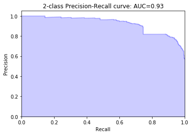
Voting Model: Curves
import matplotlib.pyplot as plt

precision, recall, prc_thresholds = precision_recall_curve(voting_predict)
average_precision = average_precision_score(voting_predict)

plt.figure()
plt.step(recall, precision, color='b', alpha=0.2,
         where='post')
plt.fill_between(recall, precision, step='post', alpha=0.2,
                 color='b')

plt.xlabel('Recall')
plt.ylabel('Precision')
plt.ylim([0.0, 1.05])
plt.xlim([0.0, 1.0])
plt.title('2-class Precision-Recall curve: AUC={0:0.2f}'.format(
          average_precision))
plt.show()
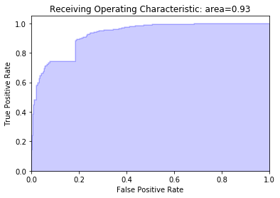
fpr, tpr, roc_thresholds = roc_curve(voting_predict)
area = roc_auc_score(voting_predict)

plt.figure()
plt.step(fpr, tpr, color='b', alpha=0.2,
         where='post')
plt.fill_between(fpr, tpr, step='post', alpha=0.2,
                 color='b')

plt.xlabel('False Positive Rate')
plt.ylabel('True Positive Rate')
plt.ylim([0.0, 1.05])
plt.xlim([0.0, 1.0])
plt.title('Receiving Operating Characteristic: area={0:0.2f}'.format(
          area))
plt.show()
Considered a bad idea to actually adjust predictions based on optimal Threshold from holdout test data curves - it's a form of overfitting on the test set: https://stackoverflow.com/questions/32627926/scikit-changing-the-threshold-to-create-multiple-confusion-matrixes (although using ROC to do this might be ok? or on cross-validated training data? https://stackoverflow.com/a/35300649)
Pickling the Voting Model
import pickle

print ("Exporting the voting model to model.pkl")
with open('model.pkl', 'wb') as f:
    pickle.dump(voting, f)
# load the model back into memory
print("Importing the model from model.pkl")
with open('model.pkl', 'rb') as f:
    loaded_clf = pickle.load(f)

# predict on a new sample
task_new = 'Buy ice cream'
print ('New sample: {}'.format(task_new))

# score on the new sample
features = featurize(nlp(task_new));
predict = [(l, p.prob('pos')) for l,p in zip(loaded_clf.classify_many(features), loaded_clf.prob_classify_many(features))]
print('Predicted class is {}'.format(predict[0]))
Next Steps and Improvements
- Training set may be too specific/not relevant enough (recipe instructions for positive dataset, recipe descriptions+short movie reviews for negative dataset)
- Throwing features into a blender - need to understand value of each
- What feature "classes" tend to perform the best/worst?
- PCA: Reducing dimensionality using most informative feature information
- Phrase vectorizations of all 0s - how problematic is this?
- Varying feature vector lengths - does this matter?
- Voting - POS taggers
- Combining verb phrases
- Look at examples from different quadrants of the confusion matrix - is there something we can learn?
- Same idea with the classification report
Things abandoned
See the original notebook for this section.
Wrap Up
Another way to describe this notebook: as both 1) generalizing (by devaluing specific word choice) bag-of-words using part-of-speech, and 2) enhancing n-gram (bigram) selection using syntactic dependencies.
Towards functional over topical similarity for task classification
Dependency-Based Word Embeddings by Omer Levy & Yoav Goldberg is a presentation I discovered after writing this notebook. The following hints at why the methodology in this notebook works:
- Bag-of-words contexts induce topical similarities
- Dependency contexts induce functional similarities
- Share the same semantic type
- Co-hyponyms
This duo also provided dependency-based embeddings from English Wikipedia, which is awesome - one cool extension I’d like to pursue is comparing my very manually-engineered classifiers against a classifier with these pre-trained embeddings at its core.
Demo Fridays: Redux
This notebook was used as part of my second team-wide demo - so here’s to pushing myself!
…even if it’s frankly terrifying to think about putting my name on something half-baked in front of ~40 people.
— Me, three weeks ago
Footnotes
-
Huge thanks to Michele Pratusevich for the detailed blog post on Blogging with Jupyter - I’ve been wanting to do this! Last convert: 11/13/2017. ↩

Nadja does not particularly enjoy writing about herself.