Energy and V.A.E.
29 Jun 2018
. category:
DL
.
Comments
#openai
Welcome to week 4! The end of this week marks the halfway point of my syllabus for the Scholars program (wow). Four more weeks until my final project begins!
I split my attention between learning about sequence-to-sequence (seq2seq) models and variational autoencoders (VAE), while also tinkering with my LSTM-based language model from weeks 2-3.
To skip ahead to seq2seq VAEs for text generation, click here.
‘Energy’-conditioned language model
Last week, I discussed the speed bumps I hit while trying to get the fastai library to support an additional contextual Field in my language model data. By Tuesday, I had a ContextLanguageModelLoader working, based on local modifications to fastai.nlp.LanguageModelLoader1. I can now pass extra context for my language model to condition on!
This week, I conditioned each word fed into my LSTM-based language model on Spotify’s definition of energy:
Energy is a measure from 0.0 to 1.0 and represents a perceptual measure of intensity and activity. Typically, energetic tracks feel fast, loud, and noisy. For example, death metal has high energy, while a Bach prelude scores low on the scale. Perceptual features contributing to this attribute include dynamic range, perceived loudness, timbre, onset rate, and general entropy.
Energy seemed like a great piece of context to include. I figured the perceived energy of a song would translate fairly distinctly to any writing about the song!2
To do this practically, in my model’s forward pass, I concatenated each and every word embedding with Spotify’s floating point energy value for whatever song the word helped describe. So if the word embedding size was 300, after the concat, it became 301. Then I trained on 15K reviews for 50 epochs (perplexity=130, aka not great3).
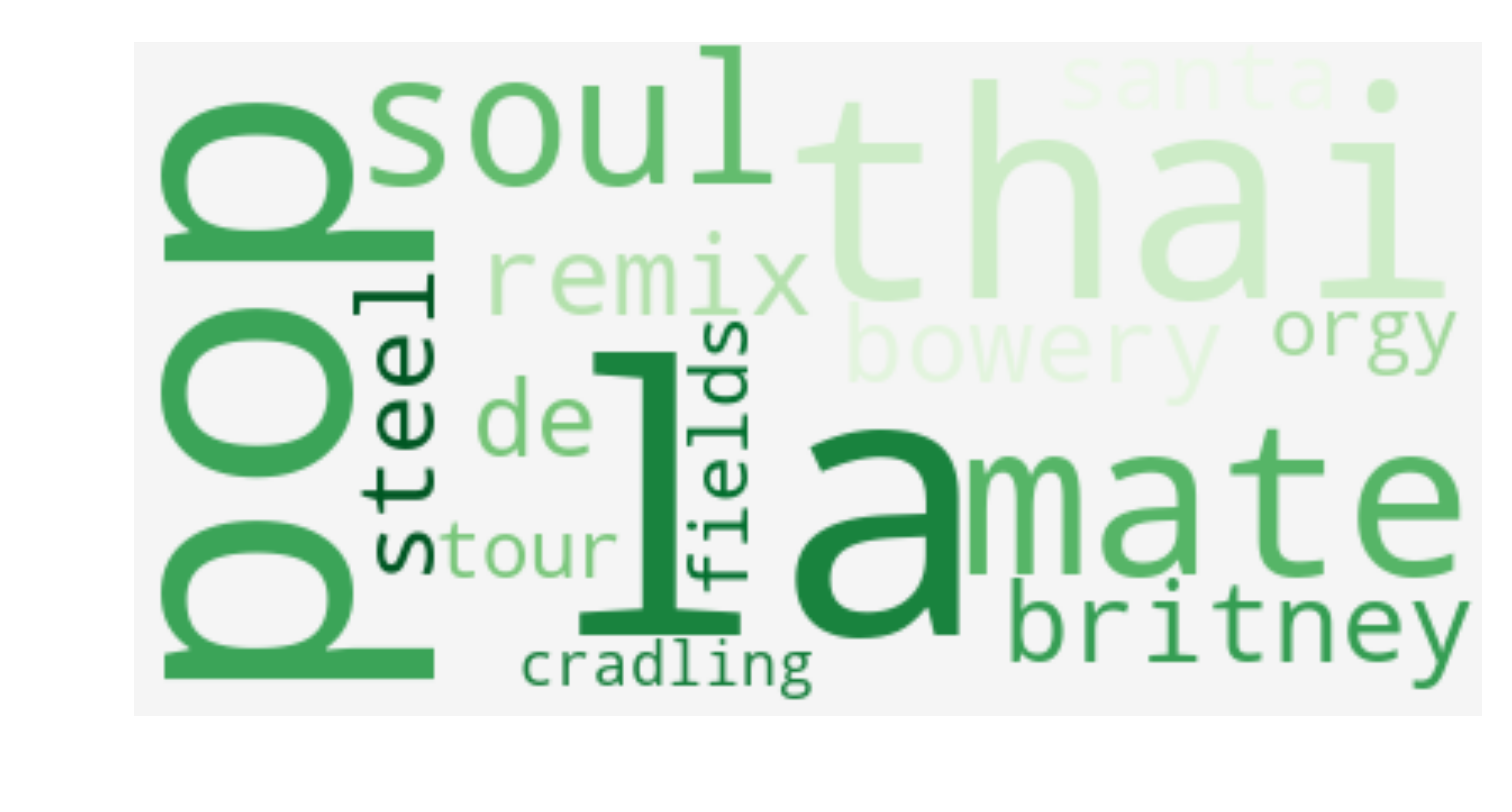
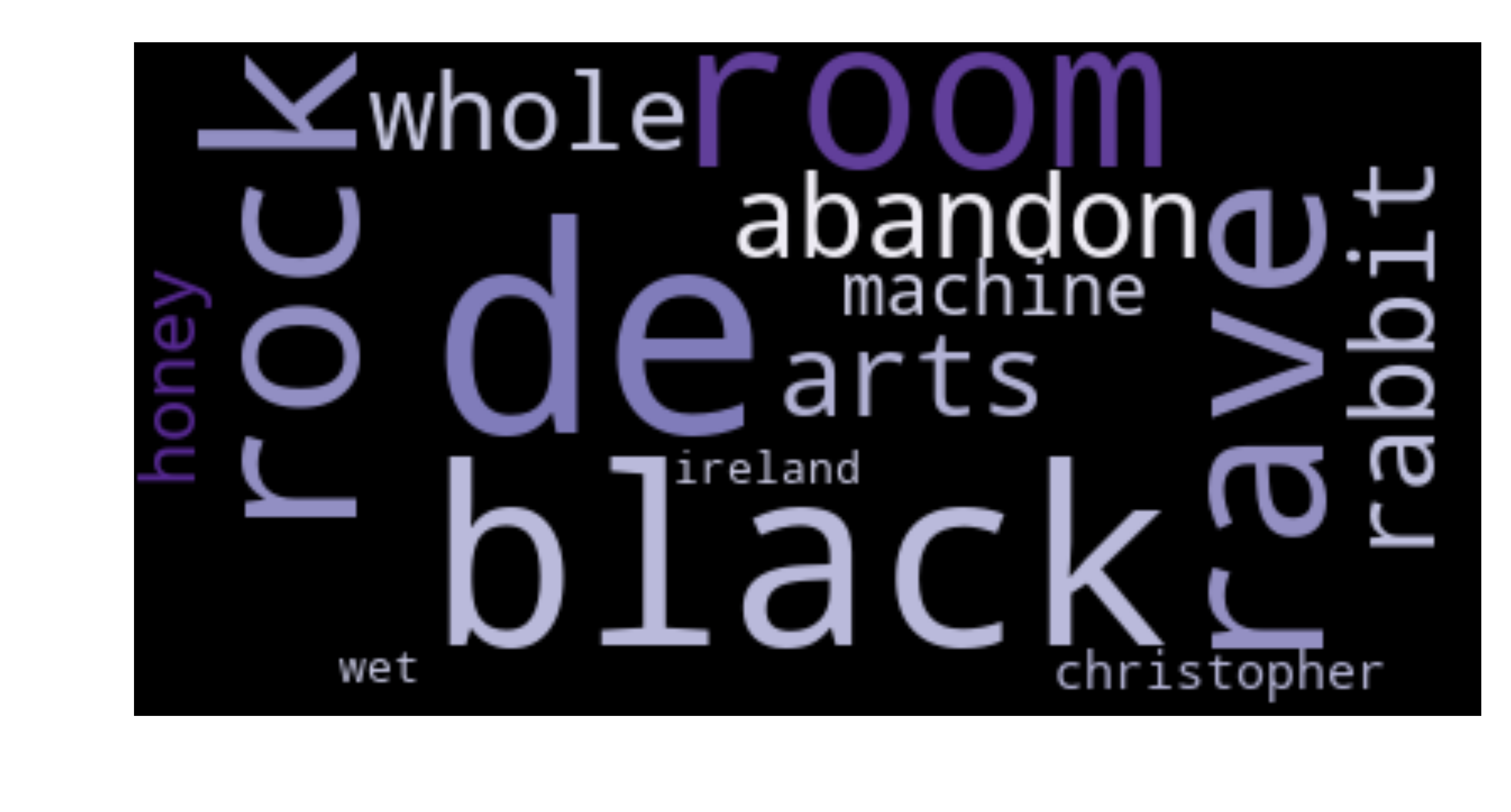
My preliminary results are pretty interesting! The generated text itself is still as garbled and hard to read as last week’s… but things get more interesting if we take a look at what words generated most frequently at the highest energy (1.0) vs. the lowest energy (0.0).
I sampled 10K words from each energy context; filtered out the NLTK English stopwords, punctuation, and numbers; then finally counted word frequencies.
| Frequent words sampled with high energy conditioning | Frequent words sampled with low energy conditioning |
|---|---|

|

|
I then immediately began speculating about what these word clouds4 could represent! Here’s a quick high energy vs. low energy comparison:
- California & Caribbean vs. Germany & Ireland
- Pop & Thai funk vs. Rock & Rave music
- Britney vs. Christopher
- Fields vs. Rooms
- Mates (friends, bonds) vs. Abandonment
Again, all pure speculation! There were also words like cradling and soul for “high energy” and whole for “low energy” that I didn’t quite associate. And there’s clearly some interesting biases going on here (e.g., location associations). But all in all, it does feel like the conditioned model learned a little extra something!
For a much more detailed analysis of the word clouds (e.g., my theory on why thai is so prevalent in “high energy”), check out the bottom of my work notebook! Can you spot any other associations?
seq2seq vae for text generation
My goal for this section was to understand what the heck a “sequence-to-sequence” (seq2seq) “variational” “autoencoder” (VAE) is - three phrases I had only light exposure to beforehand - and why it might be better than my regular ol’ language model. I also wanted to try my hand at training such a network.
I’ll give a quick overview of what I learned this week and then point towards really excellent resources that explain these concepts much better than I can.
Why?
What do I stand to gain from a seq2seq VAE, compared to the traditional LSTM language model (LSTM-LM)?
Recall that the LSTM-LM models a joint probability distribution over sequences - meaning, it models the next word in a sequence given the previous words:
[p(x) = \prod_{i=1}^{n} p(x_i \mid x_1,…,x_{i-1})]
The novelty of the network’s generations comes from sampling over all next word probabilities from the LSTM-LM’s output distribution.
However, nothing else about generating a sample produces random variability. The joint probability distribution equation above is entirely deterministic, as it is based on the sequences in the training data. It would be better for the goal of producing novel generations if I could introduce more variability to the process.
I also have a goal of producing more topical generations that capture meaning and style and other more abstract characteristics of writing. So it would be useful for the variability I introduce to still respect that the samples should have complex structure and strong dependencies.
How?
The seq2seq VAE approach promises more novel yet topical generated text. Let’s break down each part of the name.
seq2seq: a type of network where both the input and output of the network are variable-length sequences. It consists of one RNN that encodes the input sequence, then hands its encoding to another RNN which decodes the encoding into a target sequence.
- The intermediate “encoding” is known as the
thought vector(and also thehidden code/representational vector/latent vector), and it represents a compressed representation of what knowledge was needed for theencoder-decodernetwork to translate from input to target.
autoencoder: a technique that uses identical data as both the input and target data for the encoder-decoder network. The cool thing here is that, in the network’s attempt to copy the input to the target, the thought vector will become a latent (hidden) representation of the singular data provided (rather than a latent representation of some translation).
variational: a modification to the autoencoder that allows the thought vector to represent an entire distribution (rather than a fixed vector). This is cool because whenever you need a vector to feed through the decoder network, you can simply sample one (usually called z) from the thought vector distribution (encoder not required for generation!).
Put this all together and you have a network that can first learn a rich latent representation of your text, and then use that representation to generate new samples! This satisfies my more novelty goal because I can randomly sample z from the latent space of the thought vector. This satisfies my more topical goal because this thought vector must represent global properties of the text, and so using it to generate text should incorporate more abstract knowledge than the LSTM-LM can while predicting locally, word-by-word.
 An LSTM-based seq2seq VAE. Image courtesy of Bowman, S. R., Vilnis, L., Vinyals, O., Dai, A.M., Jozefowicz, R., Bengio, S (2016). Generating Sentences from a Continuous Space.
The autoencoder is such an elegant idea! Even neater, the seq2seq VAE decoder network can be thought of as a z-conditioned language model, similar to my ‘energy’-conditioned language model from part 1! z just has the potential to hold much richer knowledge than my feature-engineered choice of ‘energy.’
Resources
I had several really excellent resources to guide my learning this week.
seq2seq:
- Sutskever, I., Vinyals, O., and Le, Q. V. (2014). Sequence to sequence learning with neural networks5.
- A Practical PyTorch tutorial: “Translation with a Sequence to Sequence Network and Attention”. Even if you don’t care to implement anything in PyTorch, the words surrounding the code are good at explaining the concepts.
VAEs:
- I highly recommend this YouTube video as an “Introduction to Variational Autoencoders”!
- Once ready for some technical prose and code, check out Miriam Shiffman’s series on VAEs: an introduction and under the hood.
- For a focus on text VAEs (another paper!): Bowman, S. R., Vilnis, L., Vinyals, O., Dai, A.M., Jozefowicz, R., Bengio, S (2016). Generating Sentences from a Continuous Space.
Experiments
I also dabbled with training a seq2seq VAE. I found some code at kastnerkyle/pytorch-text-vae, updated it for Python 3 and PyTorch 0.46, and let it train!
The decoder seemed quite capable of reconstructing song titles using the hidden code. I then tried full-text song reviews… until I noticed that this encoding technique seems meant for sentence representations. It all seems to break pretty hard if you go above a sentence. The Bowman et al. paper stuck to sentence representations, and even then, it mentions:
As the sentences get longer, the fidelity of the round-tripped sentences decreases.
When I split the reviews into sentences, it then became capable of reconstructing them (makes sense as sentences are of comparable length to song titles).
The code I was using didn’t implement sampling, but it did implement something called homotopy, or the linear interpolation between sentences. From Bowman et al.:
Similarly, the homotopy between two sentences decoded (greedily) from codes
z1andz2is the set of sentences decoded from the codes on the line. Examining these homotopies allows us to get a sense of what neighborhoods in code space look like – how the autoencoder organizes information and what it regards as a continuous deformation between two sentences.
After training on review sentences for a long while, I could generate homotopies (see table below). The first column uses the same s0 and s1 as the pytorch-text-vae repo; the second column uses the same as the Bowman et al. paper.
| generated homotopy #1 | generated homotopy #2 |
|---|---|
| (s0) it had taken years to believe | (s0) he was silent for a long moment |
| (z0) it categories hip hop for something | (z0) i was working for a long moment |
| (…) it was last weekend and disco | (…) i was hell for a long moment |
| (…) it was nothing but the weekend | (…) i was me for a long moment |
| (…) it was all weekend at the end | (…) i was me in a moment |
| (z1) it was it all weekend at the end | (…) it was one in my least |
| (s1) but it was all lies at the end | (z1) did it song in my leave |
| (s1) it was my turn |
It was all weekend at the end.
Work notes
Highlights:
- Finally started using
pdbextensively this week - extremely helpful for inspecting model inputs and outputs and layer dimensions when writing theContextLanguageModelLoader
Future improvements:
- Desperately need gains in efficiency of model training. I need to break my habit of watching models train
 :
:
- parallel jobs
- hyperparameter sweeps
- organized experiments
- framework for saving and continuing training
- If I need to break all reviews into sentences to train the VAE, how do I associate each sentence with its review/song?
That’s all for this week. Next week should be a great one: all about attention!
Follow my progress this summer with this blog’s #openai tag, or on GitHub.
Footnotes
-
To see what I modified to make context work, search for
ContextLanguageModelLoaderin this notebook. ↩ -
Last week, I discussed wanting to condition on song genres. However, a quick spot check placed doubts in my mind about the accuracy of the labels I scraped from the web. So I’ve switched to energy, and I plan to condition on multiple Spotify audio features in the future. ↩
-
I haven’t mentioned perplexity since my week 1 notebook, but it’s a standard language model measure for how well a model fits a held-out text corpus. It can be calculated by taking the exponent of cross-entropy loss. SOTA (state-of-the-art) LM perplexities are between 40-70 as of writing. ↩
-
Word clouds courtesy of https://github.com/amueller/word_cloud ↩
-
Me from 4 weeks ago would have rolled my eyes and sighed at a “read this paper to get it” suggestion - but I swear the papers I’m suggesting this week are quite readable! All you need is a solid understanding of RNNs/LSTMs because they are the building blocks. ↩
