Data Is All Around Us
18 Oct 2017
. category:
Portfolio Building
.
Comments
In my first post, I mentioned having a mentor who encouraged me to build up a portfolio of at least 3 well-curated, beautiful data projects. Unsure on how to get to beautiful, I asked whether she could share any projects that I could hold as the “gold standard” while building my own portfolio.
She shared a few of her favorites on the web, mentioning that David Robinson of the Variance Explained blog has a lot of great examples.
Right now, I want to focus on one particular blog post of David’s that I admire: “Analyzing networks of characters in Love Actually”. Why? It’s a cute, simple, effective example of playing with data for neat results. I especially like his closing paragraphs on the why behind the post:
Have you heard the complaint that we are “drowning in data”? How about the horror stories about how no one understands statistics, and we need trained statisticians as the “police” to keep people from misinterpreting their methods? It sure makes data science sound like important, dreary work.
Whenever I get gloomy about those topics, I try to spend a little time on silly projects like this, which remind me why I learned statistical programming in the first place. It took minutes to download a movie script and turn it into usable data, and within a few hours, I was able to see the movie in a new way. We’re living in a wonderful world: one with powerful tools like R and Shiny, and one overflowing with resources that are just a Google search away.
Maybe you don’t like ‘Love Actually’; you like Star Wars. Or you like baseball, or you like comparing programming languages. Or you’re interested in dating, or hip hop. Whatever questions you’re interested in, the answers are just a search and a script away. If you look for it, I’ve got a sneaky feeling you’ll find that data actually is all around us.
— “Analyzing networks of characters in Love Actually” by David Robinson / CC BY-SA 4.0
Silly projects make the world go ‘round. And to me, this post is an opportunity to warm up my own skills with a remix: I am going to replicate this analysis, replacing R with Python and a Jupyter notebook, for a hands-on guided experience into great technique. I’ll also add more commentary on the smaller choices made in the project.
This will allow me to set up my coding environment, reacquaint myself with nitty-gritty R and Python, build my first Jupyter notebook1, and really understand the subtleties of the code David wrote. I’m excited, so let’s jump in!
Code
GitHub repo: https://github.com/iconix/love-actually - includes the Jupyter (Python) notebook, Shiny app code, and documentation I added to the R code.
Shiny app: https://iconix.shinyapps.io/love-actually-network/
R Walkthrough
My first pass through the R code, way back in July, was in order to understand what each line does. There was plenty unfamiliar, and the code could get dense at times. Feel free to take a look at the comments I added to David’s original R file during this process - most are about defining what different libraries and functions in R do.
From R to Python
My goal: Recreate love_actually_data.rda in Python using pandas; then convert output into .Rdata format and feed into Shiny app.
Analyzing networks of characters in Love Actually in Python
Source material in R: http://varianceexplained.org/r/love-actually-network/
David's original stated goal: "Visualize the connections quantitatively, based on how often characters share scenes."
Tasks accomplished in R:
- Organize the raw data into a table
- Create a binary speaker-by-scene matrix
- Hierarchical clustering
- Timeline visualization
- Coocurrence heatmap
- Network graph visualization
- Output data frame in a way R can consume for Shiny app usage
Tasks 1-2 are data munging/parsing/tidying. 3-6 are analysis and visualization. Task 7 is R-friendly output.
Organize the raw data into a table
Section subgoals: read in script lines; map characters to actors; transform script into a data frame with scene#, line#, character speaking, line of dialogue, and actor
David uses the R package dplyr extensively (along with a little stringr and tidyr) and in a very dense way to perform reach this goal. We'll need to unpack this in order to understand and then translate it to Python.
import os

BASE_DIR = os.getcwd() + '/..'
RAWDATA_DIR = BASE_DIR + '/rawdata'

raw_script = RAWDATA_DIR + '/love_actually.txt'
cast_csv = RAWDATA_DIR + '/love_actually_cast.csv'
from pandas import DataFrame
import pandas as pd
import numpy as np

# read in the script
with open(raw_script, 'r', encoding='utf8') as s:
    raw_df = DataFrame({'raw': s.readlines()})
raw_df[:10]
len(raw_df)
# filter out new/empty lines and lines annotated as songs
lines = DataFrame(raw_df[(raw_df.raw.str.strip() != '') & ~(raw_df.raw.str.contains('\(song\)'))])
len(lines)
lines[:10]
# mutate: add new columns to annotate scene markers and then calculate scene numbers for each line, based on markers.

lines['is_scene'] = np.where(lines.raw.str.contains("\[ Scene #"), True, False)
# fortunately, numpy has a cumsum method like R
lines['scene'] = np.cumsum(np.where(lines.raw.str.contains("\[ Scene #"), True, False))
lines[:10]
# clean up now that we're done with the is_scene column
lines = lines[~lines.is_scene] # filter out scene markers
lines = lines.drop('is_scene', axis=1) # remove is_scene column
lines[:10]
# take raw and partition by ':'
# if partition exists, left side represents the speaker, right side the dialogue of the speaker
# if partition does not exist, entire line is dialogue
raw_partitioned = lines.raw.str.rpartition(':')
lines['speaker'] = raw_partitioned[0]
lines['dialogue'] = raw_partitioned[2]
# add new column with line numbers
lines['line'] = np.cumsum(lines.speaker != '')
lines[:15]
# collapse dialogue belonging to the same line into one row:
    # group by scene and line (do not index by group labels, else we'll get a weird multi-level index at the end)
    # aggregate the dialogue across these groups (and aggregate speaker, but each line should have one speaker anyway)
lines = lines.groupby(['scene', 'line'], as_index=False).aggregate({'dialogue': lambda x: x.str.cat().strip(), 'speaker': lambda x: x.str.cat()})
lines[:10]
^Note that David did everything so far in one (extremely) dense line of R code with a bunch of piping!
# read in the character -> actor mapping
with open(cast_csv, 'r') as c:
    cast = pd.read_csv(c)
lines = lines.merge(cast)
lines['character'] = lines['speaker'] + ' (' + lines['actor'] + ')'

# clean up the output
lines = lines.sort_values('line').reset_index(drop=True)
lines[:15]
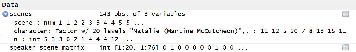
Create a binary speaker-by-scene matrix
Section subgoals: count lines per scene per character
by_speaker_scene = lines.groupby(['scene', 'character'], as_index=False).size().reset_index(name='n')
by_speaker_scene[:10]
speaker_scene_matrix = pd.pivot_table(by_speaker_scene, index=['character'],
   columns=['scene'], fill_value=0, aggfunc=np.size)
speaker_scene_matrix.shape
speaker_scene_matrix
Hierarchical clustering
Now that the data is tidy, let's begin our analysis!
First up: hierarchical clustering will provide an ordering that puts similar characters close together.
# Normalizing so that the # of scenes for each character adds up to 1 (http://varianceexplained.org/r/love-actually-network/#fn:hclust)

# in pandas, axis specifies the axis **along which** to compute
# - so we're summing along the columns (i.e. row sum) and then dividing that sum along rows ('index' in pandas)
norm = speaker_scene_matrix.div(speaker_scene_matrix.sum(axis='columns'), axis='index')
Helpful SciPy documentation:
from scipy.spatial.distance import pdist
from scipy.cluster import hierarchy

# cityblock = Manhattan distance
# complete finds similar clusters
h = hierarchy.complete(pdist(norm, metric='cityblock'))
import matplotlib.pyplot as plt

plt.figure(figsize=(12, 4))
dn = hierarchy.dendrogram(h, labels=norm.index.values, leaf_rotation=90)
plt.ylabel('cityblock distance')
plt.xlabel('hierarchy.complete(pdist(norm, metric=\'cityblock\'))')
plt.show()
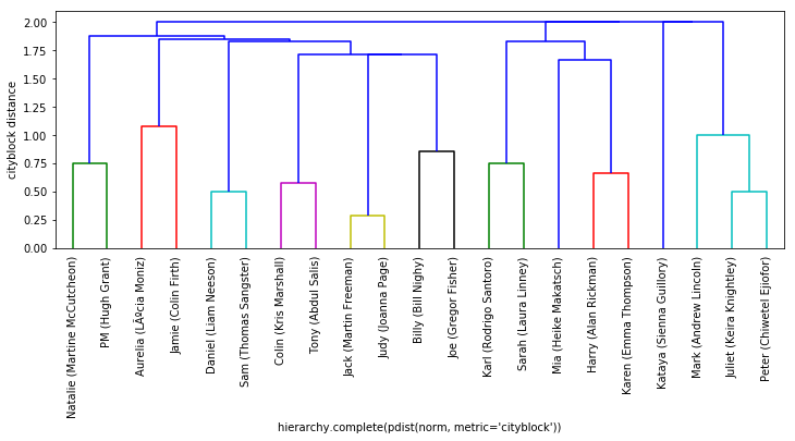
For an explanation of the y-axis value: https://stats.stackexchange.com/a/95858
I'm just going to go ahead and declare that matplotlib is prettier and more readable than R's graphics/plot package:
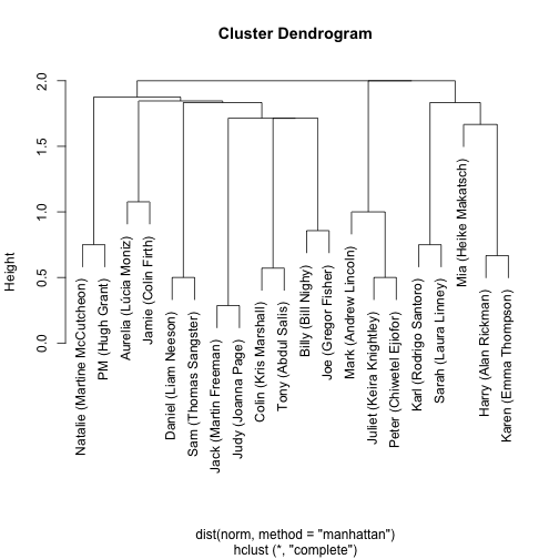
Note the differences in cluster orderings between mine and David's plots - this will account for differences in the upcoming Visual Timeline ordering as well!
EXTENSION As suggested by David, try different distance matrix computations and see what changes!
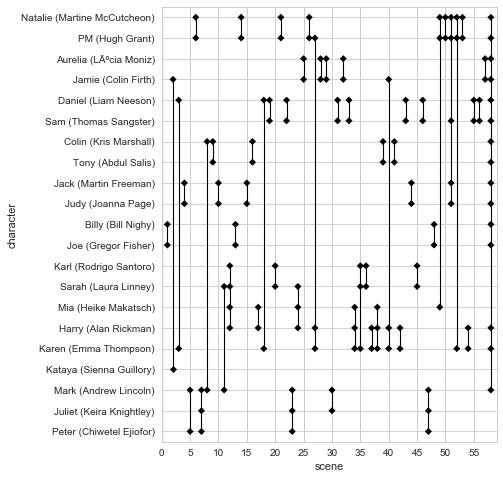
Visual Timeline
I'm excited for this visualization! It was the first one in David's original post that made me go, "huh, cool!"
scenes = by_speaker_scene.groupby('scene').filter(lambda g: len(g) > 1)
# Temporarily suppressing SettingWithCopyWarning below
original_setting = pd.get_option('chained_assignment')
pd.set_option('chained_assignment', None)
# now that we've removed scene numbers, update them so that they are contiguous integers
old_to_new_scenes = {o:n+1 for n,o in enumerate(scenes.scene.unique())}
scenes.scene = scenes.scene.apply(lambda x: old_to_new_scenes[x])
# enforce categorical ordering by character similarities found by our hierarchical clustering earlier (rather than alphabetical)
scenes.character = pd.Categorical(scenes.character).reorder_categories(dn['ivl'])
EXTENSION My initial ordering for characters as categorical data was by first appearance in movie (i.e., by scene number). The visual timeline had pretty interesting properties where you could track characters being introduced, first in pairs, then in connection with previously introduced characters.
I switched to ordering by "character similarity" to stay true to my purpose of replicating David's analysis... however, I think I like the "first appearance" ordering more! It would make the timeline more useful if you had it open during a viewing of the movie (at least during the first 25 scenes with 2+ characters).
# Turn SettingWithCopyWarning back on
pd.set_option('chained_assignment', original_setting)
ggplot for Python does not support plotting categorical variables like ggplot2 in R (https://stackoverflow.com/a/27746048), so I'm using seaborn instead: http://seaborn.pydata.org/tutorial/categorical.html
%matplotlib inline
import matplotlib.pyplot as plt
import matplotlib.ticker as ticker
import matplotlib.collections as collections
import matplotlib.colors as colors
import seaborn as sns
get_ylim_for_scene replaces David's use of geom_path(aes(group = scene) from ggplot2 to connect characters in the same scene with vertical lines.
def get_ylim_for_scene(ss, character_ordering, s):
    max_index = 0
    min_index = len(ss.scene.unique()) + 1
    for c in ss.loc[ss.scene == s].character:
        c_index = np.where(character_ordering == c)[0][0]
        max_index = c_index if c_index > max_index else max_index
        min_index = c_index if c_index < min_index else min_index
    return min_index, max_index
Now we can plot the visual timeline!
num_scenes = len(scenes.scene.unique())
num_characters = len(scenes.character.unique())

plt.figure(figsize=(6, 8))

sns.set_style('whitegrid')
timeline = sns.stripplot(x='scene', y='character', color='black', data=scenes, marker='D')
timeline.xaxis.set_major_locator(ticker.MultipleLocator(5))
timeline.set(xlim=(0,num_scenes + 1))

# inspired by: https://stackoverflow.com/a/40896356
vlines = []
for i in range(num_scenes+1):
    y_min, y_max = get_ylim_for_scene(scenes, np.array(dn['ivl']), i)
    pair=[(i, y_min), (i, y_max)]
    vlines.append(pair)

# horizontal grid lines
hlines = []
for i in range(num_characters+1):
    pair=[(0, i), (num_scenes+1, i)]
    hlines.append(pair)

hlinecoll = collections.LineCollection(hlines, colors=colors.to_rgb('lightgrey'), linewidths=1)
timeline.add_collection(hlinecoll)

vlinecoll = collections.LineCollection(vlines, colors=colors.to_rgb('black'), linewidths=1.1)
timeline.add_collection(vlinecoll)

plt.show()
Sweet!
Cooccurence Heatmap
non_airport_scenes = speaker_scene_matrix.loc[:, speaker_scene_matrix.sum(axis='index') < 10].reindex(dn['ivl'])
cooccur = np.dot(non_airport_scenes, non_airport_scenes.T)
plt.figure()
sns.heatmap(cooccur, annot=True, fmt='d', cmap='Reds', xticklabels=dn['ivl'], yticklabels=dn['ivl'])
plt.show()
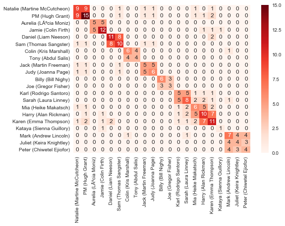
Another way to view the character clusters; I'm especially fond of the prominence of the Karl/Sarah/Mia/Harry/Karen and Mark/Juliet/Peter clusters.
I toyed with the idea of removing the info on the diagonal of 'characters in scenes with themselves' - but then I noticed that it tells how many total scenes a character is in, which is interesting to see.
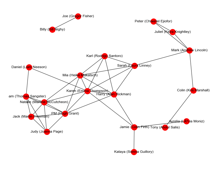
Network Graph
import networkx as nx
import pylab

def show_graph_with_labels(adjacency_matrix, mylabels):
    plt.figure(figsize=(12, 10))
    rows, cols = np.where(adjacency_matrix > 0)
    edges = zip(rows.tolist(), cols.tolist())
    gr = nx.Graph()
    gr.add_edges_from(edges)
    nx.draw_networkx(gr, node_size=400, labels=mylabels, with_labels=True)
    limits=pylab.axis('off') # turn off axis
    plt.show()

show_graph_with_labels(cooccur, dict(zip(list(range(len(dn['ivl']))), dn['ivl'])))
From Python to Shiny App
The Shiny app runs off of love_actually_data.rda, which is conventionally generated by R. Here, we will generate it with Python.
speaker_scene_matrix.columns = speaker_scene_matrix.columns.droplevel() # drop 'n'
speaker_scene_matrix.shape
scenes.shape
#!conda install rpy2
# + Add C:\..\Anaconda3\Library\mingw-w64\bin to PATH (https://github.com/ContinuumIO/anaconda-issues/issues/1129#issuecomment-289413749)
# https://stackoverflow.com/a/11586672
# http://pandas.pydata.org/pandas-docs/version/0.19.2/r_interface.html#rpy-updating

from rpy2.robjects import r, pandas2ri, numpy2ri
pandas2ri.activate()
numpy2ri.activate()

r_speaker_scene_matrix = numpy2ri.py2ri(speaker_scene_matrix.values)
r_scenes = pandas2ri.py2ri(scenes)
# bug fix for py2ri_pandasseries, which calls do_slot_assign before FactorVector for category dtype and breaks things:
# https://github.com/randy3k/rpy2/blob/master/rpy/robjects/pandas2ri.py
from rpy2.rinterface import StrSexpVector
r_scenes[1].do_slot_assign('levels', StrSexpVector(scenes.character.cat.categories))
r.assign("speaker_scene_matrix", r_speaker_scene_matrix)
r.assign("scenes", r_scenes)
r("save(speaker_scene_matrix, scenes, file='love_actually_data.rda')")
Shiny App
Here is the grande finale output of this code - try hovering over the nodes and moving the slider around!
R Tips
1. Environment setup
For understanding David’s script, I already had R and RStudio installed from an intro course I took on R. Note that the installr package (I reference it later) recommends usage through RGui rather than RStudio. Since it wasn’t obvious to me, RGui is the default R console that comes with your R installation. (I went back to RStudio after running installr.)
2. Error: package or namespace load failed for ‘dplyr’
I took the preceding Warning: package ‘dplyr’ was built under R version 3.2.5 as a hint to update my version of R from 3.2.3. I’m unsure if this affects all Tidyverse libraries, but after the update to 3.4.1 (using the installr package), I had no other installation issues.
3. ? for R’s built-in help files
My first instinct was to Google libraries and functions that I didn’t recognize, but that didn’t always return anything definitive. Then I remembered the power of the ?. It is especially hard in R to track which functions comes from what libraries, but the help files can tell you.
> ? data_frame
4. Install libraries with install.packages()
I forgot and had to look up this command.
Footnotes
-
When I first started drafting this post on 4th of July weekend, I had no hands-on experience with Juypter. The fast.ai coursework I started in mid-July changed that and helped clear up the “where to start?/where is Python now?” questions I had initially. I got caught up in various other efforts, big and small - but I’m here now to finally complete this post. ↩
-
Embed via
jupyter nbconvert --config scripts/nbconvert_config.py ../love-actually/python/love-actually.ipynb↩

Nadja does not particularly enjoy writing about herself.