Interpreting with Attention and More

This week, I picked up from last week’s study of attention and applied it towards model interpretability, or the ability for humans to understand a model. I also explored some other “attribution-based” methods of interpretability that credit different parts of the model input with the prediction.

To skip ahead to interpreting with attention, click here. Also skip ahead to interpreting with LIME, input gradients, or RNN cell activations.

Insights from explanations

This is the first of the 2 weeks I plan to spend on the subject of model interpretability, so I must think it’s pretty important (UPDATE: second week post is now live!). Deep learning models have the reputation of being inscrutable “black boxes” because their problem-solving abilities can feel almost magical.

Even now, with all of the hype and effort being applied towards deep learning, little theory about why these networks work so well exist. There’s a surprising amount of intuition and guesswork going around for a bunch of researchers and engineers. This leaves room for doubt, especially when deploying these models into the real world.

So why interpret?

• debugging/diagnosis
• trust/confidence in decisions
• real-world applicability
• detecting bias

Attention

Attention is computed as part of the network learning how to accomplish its task, which makes it very appealing as a method of interpretability. Colloquially, it tells us what the model is “paying attention” to at each time step - however, there’s evidence that it can also learn more complicated relationships that aren’t as immediately interpretable.

textgenrnn implements a weighted average attention layer at the end of its LSTM-LM. I modified the library slightly to output the attention weights at every generation time step. Then I trained the network on my song reviews dataset for 10 epochs, sampling after every 2 epochs. The heatmaps are from the attention weights used during sampling.

Here’s how attention shifts as the model generates the (cherry-picked) phrase

“a nice reminder of summer”:

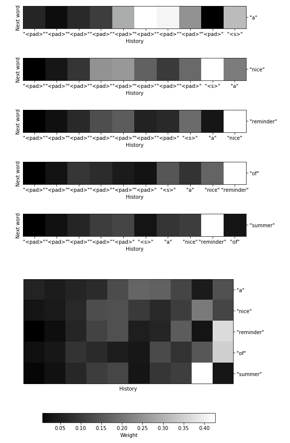
One can infer that the network paid close attention to the recently generated “reminder” when generating both “of” and “summer”, and earlier to “nice” when generating “reminder”. The model seems to pick up on a nostalgia for summer among music writers, which is pretty neat!

It’s surprising to me that so much attention is paid to the <pad> tokens, particularly early on. I was expecting the model to learn to ignore them and instead focus on <s> and eventually actual words as they slide into history. I did not train the model for long, however.

My program mentor Natasha also noticed that the model seems to latch on to particularly unique or salient words using the attention mechanism.

For instance, in sampling the phrase:

“from uk producer joe goddard , which was released earlier this year and now the”,

the network attends to “joe goddard” (and particularly “goddard”) for a long time:

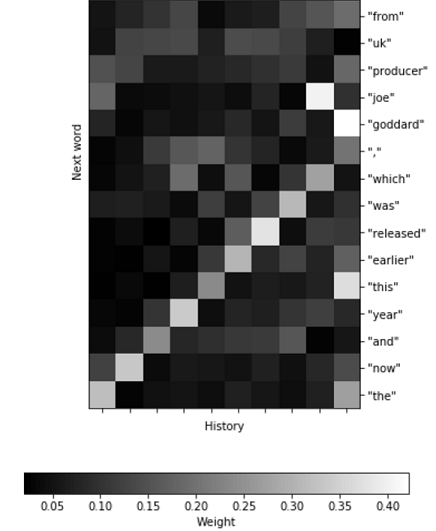
It is possible that the model is attending to words with a high TF-IDF score, which would be quite interesting! TF-IDF, or term frequency-inverse document frequency, is a measure of how unique a term is to a document. It is popularly used to reflect word importance.

For more generations and attention heatmaps, check out my work notebook.

Perturbations

I also explored assigning credit for a model prediction with input perturbations. This involves making slight changes to the input and observing how this affects the prediction.

These methods are usually applied to interpreting classification problems, which provide a nice test bed for detecting meaningful changes in the output. In particular, I looked at methods known as LIME and input gradients.

LIME

Local Interpretable Model-agnostic Explanations

LIME perturbs the input by selectively masking words in the input, then fitting a linear model. Note that local here means it interprets individual inputs and predictions, rather than making observations that hold globally for the model. From the project README:

“Intuitively, an explanation is a local linear approximation of the model’s behaviour. While the model may be very complex globally, it is easier to approximate it around the vicinity of a particular instance.”

The Anchor and SHAP (SHapley Additive exPlanations) projects are improved, generalized versions of LIME.

Below, we can see LIME provide some insight into why my movie sentiment classifier from last week incorrectly classifies the phrase, “Not once does it come close to being exciting.” as a neutral statement:

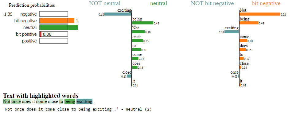
Unfortunately, because these explanations require multiple runs of the algorithm with slightly different inputs, it is computationally expensive to use. It also does not handle noise or surprise well.

Input gradients

Interpretability through input gradients uses backpropagation as a different kind of perturbation - one of infinitesimal changes.

This technique uses stochastic gradient descent (or another optimization method) on the input to the network. Like LIME, we want to see how changing the input affects network outputs. However, this technique can be used to generate an input that causes some output or neuron in the network to fire maximally.

To do this, the weights of a network are held frozen while we try to maximize the output by performing SGD on the input. This could allow us to see, for example, what input would cause the model to maximally classify a piece of text as having positive sentiment.

Ross et al. of the Right for the Right Reasons: Training Differentiable Models by Constraining their Explanations paper also provide the intuition that the input gradients themselves help define the classification decision boundary and lie normal to it. So when you look at the gradients of the probability of the predicted class, we see it will maximize by moving away from the decision boundary:

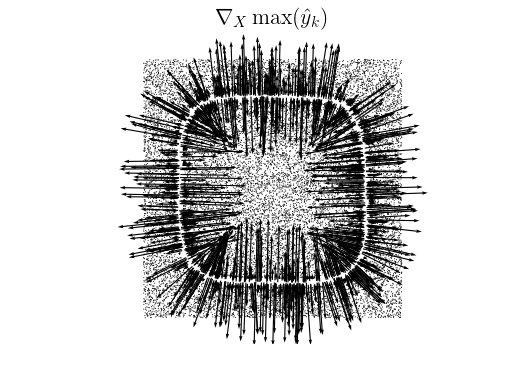
Here is an example of input gradients in action from the “RRR” paper. They even directly compare their technique to LIME:

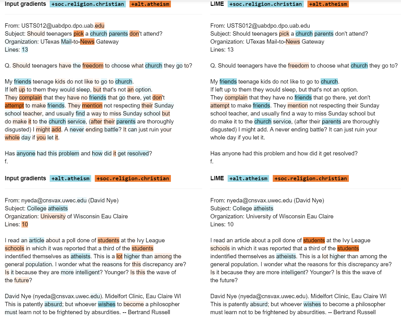
It turns out that the explanations provided by input gradients are very similar to those of LIME – input gradients are just much more computationally efficient, as well as less sparse about assigning credit. Practically however, the LIME library is more polished and easier to use.

RNN cell activations

Karpathy et al. explored the concept of “interpretable activations” in the paper Visualizing and Understanding Recurrent Networks. They liken these interpretable activations to neurons firing at different rates in the brain as it processes the input.

From “The Unreasonable Effectiveness of Recurrent Neural Networks”, Karpathy was able to find a recurrent cell in a trained LSTM that turns on only when there is an open quote that hasn’t been closed, effectively keeping track of the fact that a closing quote still needs to happen – very cool! He found another LSTM cell that similarly only turns on when inside of a coding if-statement.

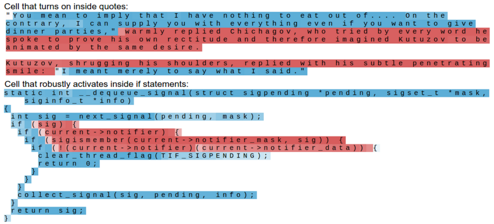
Karpathy also makes the point that many/most activations are not easily interpretable – meaning one has to manually search for ones like the “quotes cell” that are.

Follow my progress this summer with this blog’s #openai tag, or on GitHub.