Training an LC-GAN
28 Jul 2018
. category:
DL
.
Comments
#openai
I spent the last week before my 4-week final project understanding, implementing, and training a special kind of GAN. GAN is short for generative adversarial network, a neural network that “simultaneously trains two models: a generative model G that captures the data distribution, and a discriminative model D that estimates the probability that a sample came from the training data rather than G” (from the original GAN paper).
In other words, the generator G is trained to fool the discriminator D, while D is trained to learn how to distinguish between real and fake (G) samples. In this way, the two models are adversaries.
Adversarial training has been somewhat famously called “the coolest idea in machine learning in the last 20 years.”

LC-GAN
Quick note: if a quote in this post appears unattributed, it is most likely from Engel, J., Hoffman, M., Roberts, A. (2017). Latent Constraints: Learning to Generate Conditionally from Unconditional Generative Models.1
Architecture
I focused on training a particular type of GAN to learn latent constraints (LC-GAN) as a way of conditioning the generations of my pretrained seq2seq VAE from weeks prior. This direction was inspired by work my program mentor Natasha Jaques did previously to improve the generative sketching model Sketch RNN with facial feedback.
Engel et al. describe latent constraints as “value functions that identify regions in latent space that generate outputs with desired attributes.” These constraints enable a user to fine-tune a VAE model to generate samples with specific attributes, all the while preserving each sample’s core identity. Like the ULMFiT approach from week 5, adding latent constraints involves a fine-tuning procedure, so 1) no retraining is required, and 2) compared to training from scratch, a much smaller labeled data set (or rules-based reward function) is needed. For example, Natasha was able to produce pleasing sketch samples from ~70 samples per sketch class.
The latent constraints can be broken down into two subcategories - the realism constraint and the attribute constraints.
- Realism “enforces similarity to the data distribution” so that samples look realistic. This constraint is implicitly satisfied by training a GAN discriminator to differentiate between thought vectors
zfrom real training samples and randomzfrom the Gaussian (normal) distribution. - Attribute constraints are what allow the user to control the attributes exhibited by the samples. This constraint is conveyed through a user-provided labeled data set or reward function that lets another GAN discriminator know what constitutes a satisfying sample.
Such latent constraints can be learned from the following GAN architecture:

D training, and the center green box represents generator G training. The blue boxes along the sides show the internal architectures of G and D - both are similar, except G's final layer is a gating mechanism that allows the generator to remember/forget what it wants about the z it was provided as input and the z it computed with its own layers.
Not pictured above is the precursory step where the user produces the correct labels v for discriminator training.
There are hints at the training procedure in the diagram as well - let’s discuss training details more.
Training procedure
The grey column in the middle of the diagram above represents the training loop. An iteration consists of M batches of discriminator D training, followed by N batch of generator G training, where M >> N. We intentionally train D a lot more than G because the generator is very sensitive to overtraining.2
The z input into D comes from the pretrained VAE (satisfying the realism constraint). The v output by D is then compared to the correct v (as rewarded or labeled by the user) using cross-entropy loss.
The z ~ N(0,1) input into G is “noise” from a random Gaussian (normal) distribution. The generator is meant to turn this noise into a z_prime that is able to produce a good sample. The z_prime output by G is then fed into D, which produces a label v that is then used directly as the loss to judge whether G indeed produced a sample that satisfy the user’s attribute constraints.
As Jaques et al. state, “because the latent space of a VAE is already a small-dimensional representation, it is straightforward to train a discriminator to learn a value function on z, making the LC-GAN well-suited to learn from small sample sizes.” This makes LC-GAN training fast (computationally inexpensive) and straightforward, which is a welcome change of pace from the RNN and VAE training I’ve been doing all summer long.
Why this works well
There are some really interesting concepts around why VAEs and GANs can work together like this.
Both VAEs and GANs are considered deep latent-variable models because they can “learn to unconditionally generate realistic and varied outputs by sampling from a semantically structured latent space” (Engel et al.). This structure is what the latent constraints aim to manipulate towards more “satisfying” samples.
VAEs and GANs also have complementary strengths and weaknesses:
- GANs suffer from mode collapse. This is “where the generator assigns mass to a small subset of the support of the population distribution,” effectively missing out on generating a plurality of realistic samples.3
- VAEs suffer from a blurriness tradeoff. They can “either produce blurry reconstructions and plausible (but blurry) novel samples, or bizarre samples but sharp reconstructions” – this results in a tradeoff between good samples and good reconstructions.
For the LC-GAN, the VAE should be trained to achieve good reconstructions, at the expense of good sampling. There are a few reasons for this:
- Good reconstructions allow the core identity of a sample to be preserved, even during attribute transformations.
- Good reconstructions also ensure realism.
- Realism, in turn, sharpens samples, helping to “close the gap between reconstruction quality and sample quality (without sacrificing sample diversity).”
And once good reconstructions enable attribute constraints, attribute constraints become “identity-preserving transformations that make minimal adjustment in latent space” - which helps the GAN avoid mode collapse and encourage diverse samples. The symbiotic relationship between a pretrained VAE and a finetuning GAN is pretty remarkable!
Here is a telling visual from the Engel et al. paper that really highlights the tradeoff between good reconstructions and good samples:
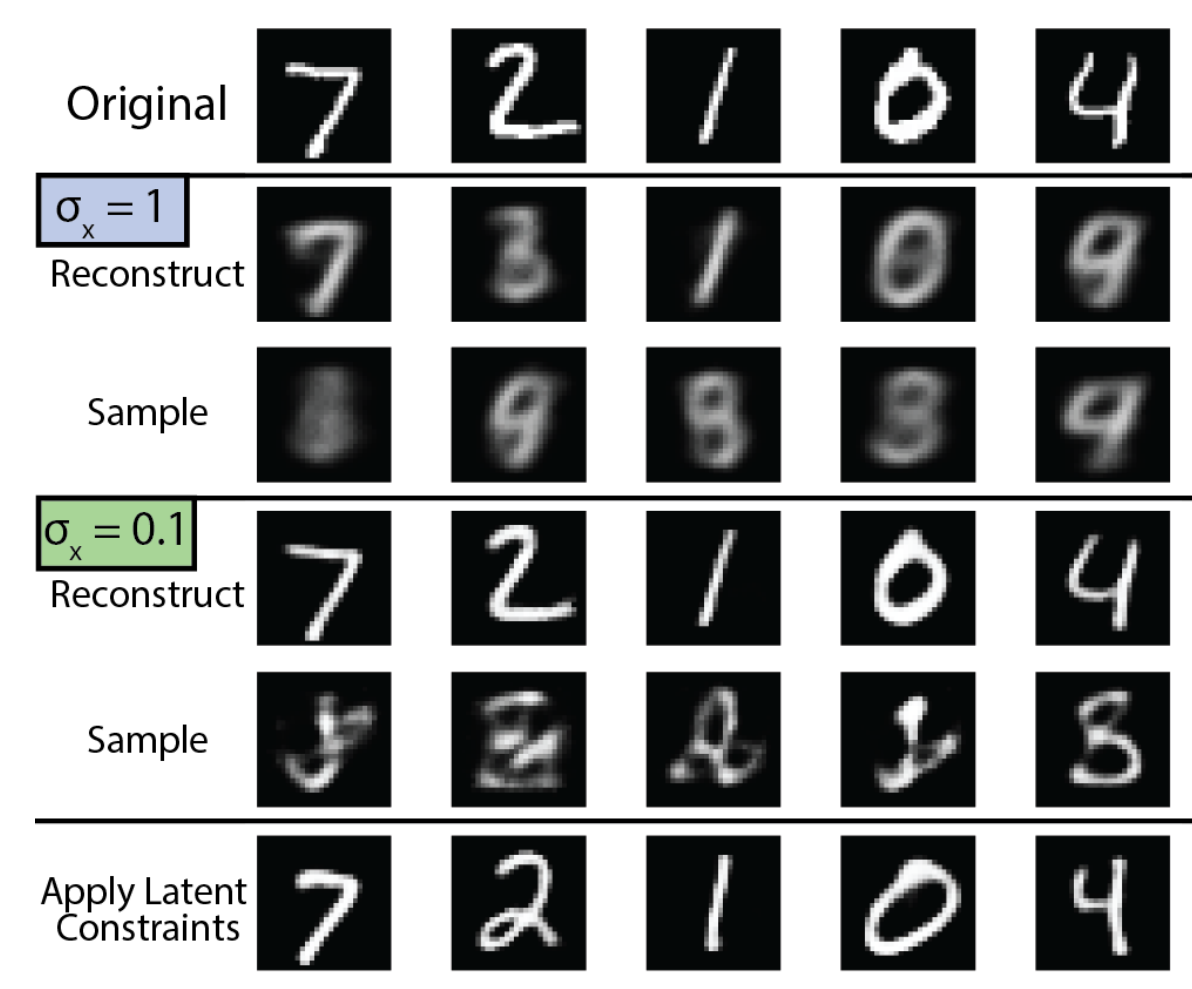
sigma_x = 1, this VAE trained on MNIST produces "coherent samples at the expense of visual and conceptual blurriness." At sigma_x = 0.1, this VAE "increases the fidelity of reconstructions at the cost of sample realism." However, applying latent constraints on the VAE at sigma_x = 0.1 can "shift prior samples to satisfy the realism constraint, [achieving] more realistic samples without sacrificing sharpness." Image from Engel et al.
Why GANs on text are hard
So perhaps I’ve made it seem like applying GANs to NLP problems is easy, but this is not actually the case generally.
Discrete sequences, like text, have a non-differentiable decoder: the output is sampled over a distribution of words. This sample cannot be back-propagated through, as is.
For an impassioned, contentious commentary on the state of GANs for NLP, and deep learning for NLP in general, see Yoav Goldberg’s Medium post “An Adversarial Review of ‘Adversarial Generation of Natural Language’” - and be sure to check out the updates as well.
We get around this differentiation problem here because we are back-propagating the gradients through thought vectors z and not text.
Follow my progress this summer with this blog’s #openai tag, or on GitHub.
Footnotes
-
If interested, the paper is accompanied by a Google Colab notebook. ↩
-
This is because too much training can lead to
Ggenerating samples way out of the Gaussian distribution expected by the decoder, resulting in bizarre results. ↩ -
Natasha shared a blog post with me on “KL-divergence as an objective function” – and I bring it up now because it turns out that GANs implicitly fit to an exclusive KL objective. If you look at the exclusive KL graph in the blog post, you can get an intuitive sense for why mode collapse happens in GANs - note how the true distribution
Phas two centers of mass, and yetQ(and thus GANs) overfits to just one of them. To contrast, VAEs optimize for inclusive KL, so it seeks the mean and ends up not fitting either center well at all; even worse, it hallucinates mass in between the two centers. Another contrasting relationship between VAEs and GANs! ↩

Nadja does not particularly enjoy writing about herself.